Models to understand and explore dynamic systems.
The examples presented here illustrate different possibilities offered by TempReas, from simple models to more complex simulations.
Example: Transition of a Vehicle Fleet
How can the gradual transition from a gasoline vehicle fleet to an electric vehicle fleet be modelled while maintaining a constant tax revenue?
In this example, the model starts with 10,000 gasoline vehicles. Each month, 2% of the remaining fleet is transferred to the electric fleet.
The initial tax revenue is €360,000 per month. As the gasoline fleet decreases, TempReas automatically calculates the electric revenue required to maintain this constant revenue, and then determines the corresponding tax per kilometer.
This example shows in particular how stocks, flows and their dependencies can be used to progressively build a dynamic model.
Taxation and Repair
This model studies the influence of taxation on repair and replacement behavior for electronic devices.
It represents the evolution of a fleet of devices over time, taking into account repairs, purchases of new devices and devices reaching the end of their useful life.
Several repair taxation scenarios can be compared in order to observe their consequences on device usage, fleet renewal and electronic waste generation.
The objective is to study, over a long period, how different levels of taxation on repair can influence the choice between repairing an existing device and purchasing a new one.
The simulation makes it possible to observe the cumulative effects of these choices on the evolution of the device fleet and on the flows associated with renewal and end of life.
The model makes it possible to compare several scenarios corresponding to different VAT rates applied to repair.
The results make it possible to compare the evolution of the system over time and analyze the consequences of each scenario.
Two documents present this model and the results obtained from the simulations:
These documents provide details on the construction of the model, its parameters, the scenarios studied and the results of the simulations.
Transfer between two stocks
This example presents a simple model in which a flow progressively transfers part of the value of one stock to another.
It illustrates the principles of model construction, its evolution over time, dynamic graphical visualization, and the consultation of calculated results.
The model consists of two stocks connected by a transfer flow.
The Stock source receives an initial allocation of 1000, while the Stock destination is initialized to 0.
The Transfert flow contains an action that defines its value at each unit of time:
y = Svalue("Stock source") * 0.1The flow therefore depends directly on the value of the Stock source: at each unit of time, it transfers 10% of this value to the Stock destination.
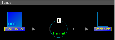
After compilation, TempReas directly displays the results within the model.
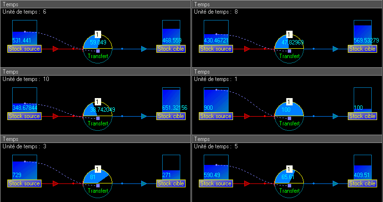
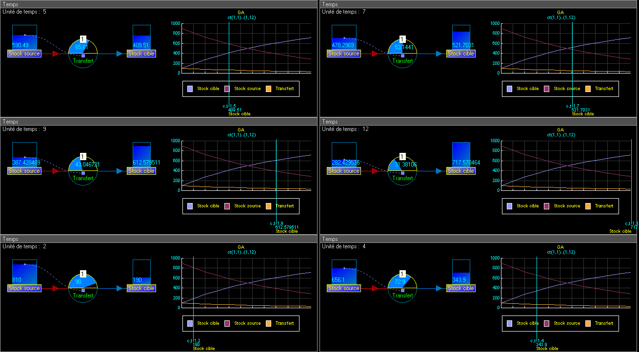
As the time unit changes, the values of the stocks and the flow are updated. The graphical representation of the stocks also changes according to their values.
The dependency relationship created by the
Svalue() call is graphically represented between
the flow and the Stock source. It accompanies the evolution
of the model over time.
The information panel indicates the current time unit, making it possible to simultaneously follow the evolution of the model and the simulation time.
The graph represents the evolution of the selected elements over the simulated period.
Its cursor is synchronized with the current time unit of the model. As time advances, the cursor moves simultaneously on the graph and in the model visualization.
The values corresponding to the selected point in time can therefore be directly related to the state of the model.
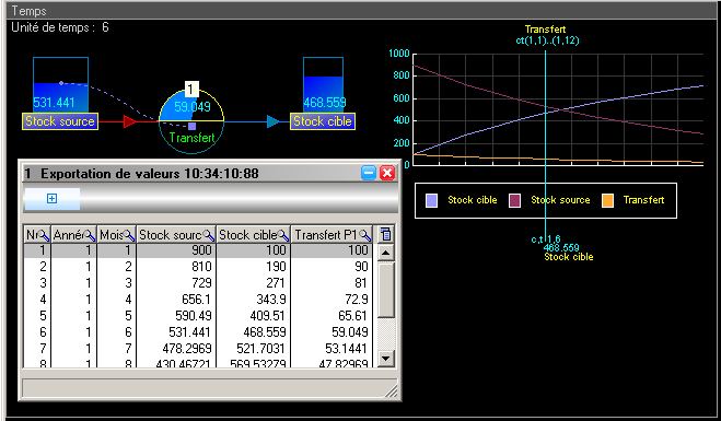
The results of the selected elements can be viewed as a table over all or part of the simulated period.
The table contains one row for each time unit and one column for each selected element. The first columns indicate, in particular, the cycle and the time unit.
The selected rows can then be exported to different formats: Excel, Word, XML or TXT, making it possible to continue the analysis with external tools.
Working with vectors.
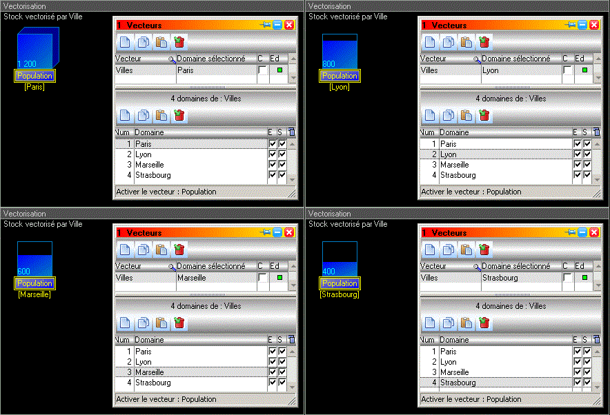
TempReas allows an element to be vectorized so that several domains can be associated with it and a specific value can be defined for each of them.
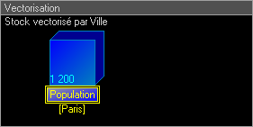
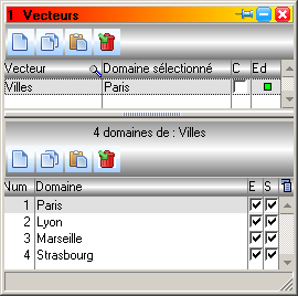
In this example, the Population stock is vectorized by the Ville vector. The stock retains a default value, but this value can be replaced by an initial allocation specific to each domain of the vector.
Selecting a domain in the vector window then makes it possible to directly display, in the model, the value corresponding to that domain.
Vectorizing a flow with a stock.
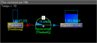
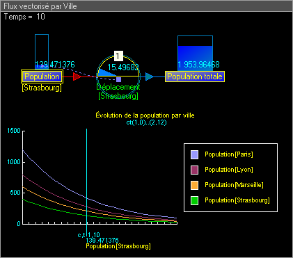
Vectorization can also be extended to flows that connect the elements of a model.
In this example, the Population stock and the Déplacement flow are both vectorized by the same Ville vector.
The flow then uses, for each city, the corresponding value of the Population stock. Each component therefore evolves independently during the simulation.
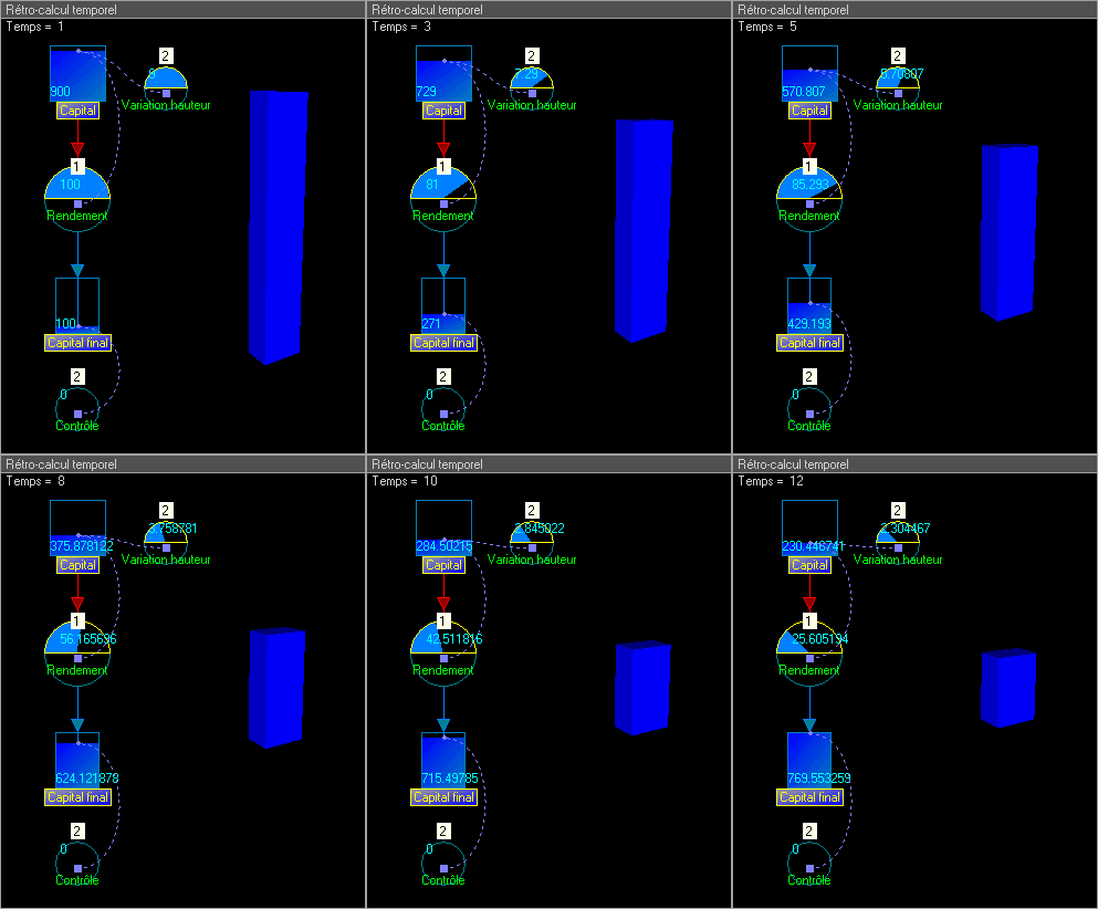
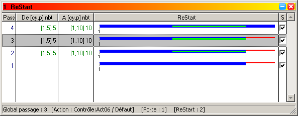
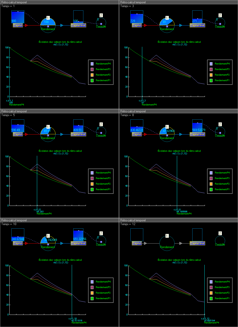
Going back in time to recalculate.
TempReas allows the calculation to be resumed at an earlier time unit in order to study the consequences of a modification on the remainder of the simulation.
The ReStartAt() function provides a way to go
back in time. The calculation then resumes at the requested
point before continuing again towards the present.
The different calculation runs performed during a backward recalculation are retained by TempReas and can be viewed and selected for the display of results.
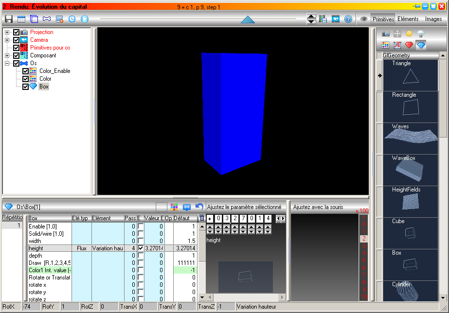
Visualizing a model in three dimensions.
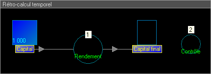
TempReas allows three-dimensional renderings to be integrated directly into a model and to evolve according to the values calculated by the simulation.
In this example, the value of Capital determines that of the virtual flow Variation hauteur. This value is directly associated with the Height parameter of a 3D primitive.
The height of the object therefore changes automatically during the simulation, according to the evolution of the model.